Thermo Exam

This example is a full thermodynamics exam that showcases pygacity’s integration with the sandler ecosystem of Python packages (sandlerprops, sandlersteam, sandlerchemeq). Compared to the Compound Exam example, it introduces:

• Steam property look-ups via SANDLER(T=..., P=...)

• pint-aware answer registration — AnsSet.register accepts pint.Quantity values and stores the magnitude and unit string automatically

• Matplotlib figure generation inside a pythontex pycode block

• Chemical equilibrium calculations via ChemEqSystem, with LaTeX output produced by the texgen_kacalculations, stoichiometrictable_as_tex, and thermochemicaltable_as_tex monkeypatches

All files are in the examples/thermo_exam/ directory:

thermo_exam/
├── ThermoExam.yaml          # pygacity configuration
├── air_mixing.tex           # Problem 1: ideal-gas mixing (30 pts)
├── desuperheater.tex        # Problem 2: steam desuperheater (20 pts)
├── vle_binary_OCM.tex       # Problem 3: binary VLE + figure (20 pts)
└── ammonia_synthesis.tex    # Problem 4: chemical equilibrium (30 pts)

The Configuration File

document:
  preamble:    
    commands:
      Universityname: University of Nowhere
      Departmentname: Mechanical Engineering
      Instructorname: Eustace T. Smartypants
      Instructoremail: ets@unow.edu
      Coursename: BIO 5678 - Applied Pyrohydrodynamics
      Termcode: 202525
      Termname: Winter 2025-2026
  structure:
    - pythontex:
        - setup
        - matplotlib
        - sandler
    - text: |
            \examheader{Exam I}{January 13, 2026}
            \noindent\textbf{Instructions:} This exam is closed book, and you are allowed 
            3 pages of your own handwritten notes on paper.  No electronic devices except 
            for a non-smartphone, non-tablet based calculator. Show all work for full credit. 
            Clearly indicate your final answers. The total number of points is 100. You have 
            110 minutes to complete the exam.
    - question_number: 1
      source: air_mixing.tex
      points: 30
    - question_number: 2
      source: desuperheater.tex
      points: 20
    - question_number: 3
      source: vle_binary_OCM.tex
      points: 20
    - question_number: 4
      source: ammonia_synthesis.tex
      points: 30
    - pythontex:
      - showsteamtables
      - teardown
build:
  seed: 12345
  copies: 30
  bundle-size: 10
  two-sided: false
  serial-hex: true
  job-name: ExamI
  paths:
    build-dir: ./build

A few points of interest:

Three pythontex blocks are listed at the top of the document structure: setup, matplotlib, and sandler. The sandler block imports the full sandler ecosystem into the pythontex session — including SandlerSteamState as SANDLER, Component, Reaction, ChemEqSystem, the sandlerprops compound database as SandlerProps, and all monkeypatches that add LaTeX-generation methods to those classes.

Header substitutions — the header.tex preamble accepts course-specific strings (university name, course number, instructor, date) via the top-level substitutions map, making it straightforward to reuse the same exam template across courses.

Problem 1: Ideal-Gas Mixing (air_mixing.tex)

\begin{pycode}
MIXER = Pick.pick_state(
    dict(
        P1={'default':14,'pick':{'between':[13,15],'round':2}, 'units': ureg.bar},
        P2={'default':12,'pick':{'between':[10,12.5],'round':2}, 'units': ureg.bar},
        T1={'default':1000,'pick':{'pickfrom':[900,950,1000,1050,1100]}, 'units': ureg.K},
        T2={'default':400,'pick':{'pickfrom':[350,375,400,425,450]}, 'units': ureg.K},
        T3={'default':600,'pick':{'pickfrom':[500,550,600,650,700]}, 'units': ureg.K},
        CP_over_R={'default':3.5,'pick':{'pickfrom':[3.0, 3.5, 4.0]}}
    )
)
P1 = MIXER.P1
P2 = MIXER.P2
T1 = MIXER.T1
T2 = MIXER.T2
T3 = MIXER.T3
CP_over_R = MIXER.CP_over_R
alpha = (T1 - T3) / (T3 - T2)
P3 = pow(pow(T3**(1 + alpha) / T1 / T2**alpha, CP_over_R) * P1 * P2**alpha, 1 / (1 + alpha))
P3 = P3.m * ureg.bar
cpr = tu.frac_or_int_as_tex(fr.Fraction(CP_over_R))

AnsSet.register(qno, label=r'\(\alpha\)', value=alpha, formatter='{:.3f}')
AnsSet.register(qno, label=r'\(P\)', value=P3, formatter='{:.3f}')
\end{pycode}
A stream of air at \pypp[0]{P1} and \pypp[0]{T1} (labeled ``stream 1'') is to be cooled to \pypp[0]{T3} by mixing with another stream of air at \pypp[0]{P2} and \pypp[0]{T2} (labeled ``stream 2'').  Let $\alpha$ be the ratio of the molar flow rate of the hotter stream to that of the cooler stream.  Compute (1) $\alpha$, and (2) the pressure $P$ of the mixed stream (labeled ``stream 3'').  You may assume this is carried out adiabatically and that air is an ideal gas for which $C^*_{\rm P}$ = $\py{cpr}R$.

It may be helpful for you to remember, {\bf for the ideal gas}, that a change of state from $(T_A,P_A)$ to $(T_B,P_B)$ results in the following enthalpy and entropy changes, respectively:

\begin{align*}
\Delta \molar{H} \equiv \molar{H}_B-\molar{H}_A = \int_{T_A}^{T_B} C^*_{\rm P} dT\\
\Delta \molar{S} \equiv \molar{S}_B-\molar{S}_A = \int_{T_A}^{T_B} \frac{C^*_{\rm P}}{T} dT - R \ln\frac{P_B}{P_A}.
\end{align*}

\ifshowsolutions\Solutionheader

Let $\dot{n}$ be the unknown molar flow rate of stream 1.  This means the outlet stream (3) has a flow rate of $\alpha\dot{n}$.  An energy balance here resolves to 
\begin{align*}
H_{\rm out} & = H_{\rm in}\\
(1+\alpha) \dot{n} \Hb(T_3,P_3) & = \dot{n}\Hb(T_1,P_1) + \alpha\dot{n} \Hb(T_2,P_2)\\
(1+\alpha)  \int_{T_r}^{T_3} C^*_{\rm P} dT & = \int_{T_r}^{T_1} C^*_{\rm P}dT + \alpha\int_{T_r}^{T_2} C^*_{\rm P}dT\\
(1+\alpha)C^*_{\rm P}(T_3-T_r) & = C^*_{\rm P}(T_1-T_r) + \alpha C^*_{\rm P}(T_2-T_r)\\
(1+\alpha)T_3 & = T_1 + \alpha T_2\\
\Rightarrow T_3 & = \frac{T_1+\alpha T_2}{1+\alpha},\ \mbox{or}\\
\alpha & = \frac{T_1-T_3}{T_3-T_2}\\
  & = \frac{\pypl[0]{T1}-\pypl[0]{T3}}{\pypl[0]{T3}-\pypl[0]{T2}} = \frac{\pypl[0]{T1-T3}}{\pypl[0]{T3-T2}} = \fbox{\pypl[3]{alpha}}.
\end{align*}
(Note all terms involving $T_r$ cancel and $C^*_{\rm P}$ divides out.).  We can get $P_3$ from an entropy balance:
\begin{align*}
S_{\rm out} & = S_{\rm in}\\
(1+\alpha)\dot{n} \Sb (T_3,P_3) & = \dot{n}\Sb(T_1,P_1) + \alpha\dot{n} \Sb(T_2,P_2)\\
\Sb(T_3,P_3) - \Sb(T_1,P_1) + \alpha\left[\Sb(T_3,P_3)-\Sb(T_2,P_2)\right] & = 0\\
C^*_{\rm P}\ln\frac{T_3}{T_1} - R\ln\frac{P_3}{P_1} + \alpha\left[C^*_{\rm P}\ln\frac{T_3}{T_2}-R\ln\frac{P_3}{P_2}\right] & = 0\\
C^*_{\rm P}\ln\left(\frac{T_3^{1+\alpha}}{T_1T_2^\alpha}\right) - R\ln\left(\frac{P_3^{1+\alpha}}{P_1P_2^\alpha}\right) & = 0\\
\ln\left[\left(\frac{T_3^{1+\alpha}}{T_1T_2^\alpha}\right)^{\frac{C^*_{\rm P}}{R}}\right] & = \ln\left(\frac{P_3^{1+\alpha}}{P_1P_2^\alpha}\right)
\end{align*}
Solving for $P_3$ gives
\begin{align*}
\Rightarrow\ P_3 & = \left[\left(\frac{T_3^{1+\alpha}}{T_1T_2^\alpha}\right)^{\frac{C^*_{\rm P}}{R}}P_1P_2^\alpha\right]^{\frac{1}{1+\alpha}}\\
& = \left[\left(\frac{(\pypl[0]{T3})^{(1+\pypl[3]{alpha})}}{(\pypl[0]{T1}) (\pypl[0]{T2})^{\pypl[3]{alpha}}}\right)^{\py{cpr}} (\pypl[0]{P1}) (\pypl[0]{P2})^{\pypl[3]{alpha}}\right]^{\frac{1}{1+\pypl[3]{alpha}}} \\
& = \fbox{\pypp[0]{P3}}.
\end{align*}
\clearpage
\else
\ifgivespace
\clearpage
\noindent (This page left blank for extra space for Problem \theenumi.)
\clearpage
\fi
\fi

This problem exercises the standard energy- and entropy-balance derivation for adiabatic mixing of two ideal-gas streams. Six parameters are picked independently per serial: two inlet pressures, two inlet temperatures, the target outlet temperature, and \(C^*_P/R\) (drawn from [3.0, 3.5, 4.0]).

Pick.pick_state controls all six at once. Note the mix of pickfrom (draws from an explicit list) and between (draws a random value in a continuous range rounded to the specified precision) strategies. The dictionary passed to Pick.pick_state also includes the units key, so the picked values are wrapped in pint units automatically (e.g. T1 = 300.0 * ureg.K) and all subsequent arithmetic carries units through to the final answers.

The outlet pressure P3 and flow-rate fraction \(\alpha\) are computed as pint.Quantity instances, which are passed to AnsSet.register. The local Python variable qno always contains the current question number. The \pypp[#]{...} inline expressions are shorthand for pythontex’s \py{...} that also detect pint.Quantity values and format them with the magnitude and unit string together. In the solution text, the same values are formatted with f-strings using use the ~P pint format specifier (e.g. f'{P1:.0f~P}') so that value and abbreviated unit string appear together in the typeset text automatically. \pppl[#]{...} is the \pypp variant that also applies the ~L format specifier, so it can be used directly in the LaTeX without needing an f-string.

Problem 2: Steam Desuperheater (desuperheater.tex)

\begin{pycode}
DSUH = Pick.pick_state(
    dict(
        P1={'default':3.2,'pick':{'between':[2.9,3.9],'round':1}, 'units': ureg.MPa}, # MPa
        T1={'default':355,'pick':{'between':[340,360],'round':0}, 'units': ureg.degC}, # C
        Psat={'default':2.9,'pick':{'between':[2.7,2.9],'round':3},'units': ureg.MPa}, # MPa
        TL={'default':50,'pick':{'between':[45,55],'round':0}, 'units': ureg.degC}, # C
        mdot={'default':15,'pick':{'between':[10,50],'round':0}, 'units': ureg.kg/ureg.s})) # kg/s
P1  = DSUH.P1
T1 = DSUH.T1
Psat = DSUH.Psat
TL = DSUH.TL
mdot = DSUH.mdot
inlet = SANDLER(T=T1, P=P1)
outlet = SANDLER(P=Psat, x=1.0)
inL = SANDLER(T=TL, x=0.0)

mLdot = mdot * ((inlet.h - outlet.h)/(inlet.h - inL.h))
AnsSet.register(qno, label=r'\(\dot{m}_\mathrm{L}\)', value=mLdot, formatter='{:.3f}')
\end{pycode}
Superheated steam at \pypp[0]{P1} and \pypp[0]{T1} is to be converted to saturated steam at \pypp[2]{Psat} in a desuperheater.  This desuperheater is supplied with inlet liquid water at \pypp[0]{TL}.  The unit should produce saturated steam at a rate of \pypp[0]{mdot}.  Assuming adiabatic operation, and assuming the liquid inlet is saturated, what is the mass flowrate of the inlet water?

The following enthalpies will be useful:
\begin{itemize}
\item[] Superheated steam at \pypp[0]{P1} and \pypp[0]{T1}: $\hat{H}$ = \pypp[2]{inlet.h};
\item[] Saturated liquid water at \pypp[0]{TL}: $\hat{H}^{\rm L}$ = \pypp[2]{inL.h}; and
\item[] Saturated water vapor at \pypp[2]{Psat}: $\hat{H}^{\rm V}$ = \pypp[2]{outlet.h}.
\end{itemize}

\ifshowsolutions\Solutionheader

Let stream 1 be the liquid water stream, which we assume is saturated liquid, stream 2 be the superheated steam inlet, and stream 3 be the saturated steam outlet.  Hence, $\dot{m}_3$ = \pypp[0]{mdot} as given.  The mass and energy balance yield the two unknowns $\dot{m}_1$ and $\dot{m}_2$:

\begin{align*}
\dot{m}_1 + \dot{m}_2 & = \dot{m}_3\\
\dot{m}_1\hat{H}_1 + \dot{m}_2\hat{H}_2 & = \dot{m}_3\hat{H}_3\\
\end{align*}

Solving these two simultaneously yields 

\begin{align*}
\dot{m}_1 & = \dot{m}_3\left(\frac{\hat{H}_2-\hat{H}_3}{\hat{H}_2-\hat{H}_1}\right)\\
& = \left(\pypl[0]{mdot}\right)\left(\frac{\pypl[2]{inlet.h}-\pypl[2]{outlet.h}}{\pypl[2]{inlet.h}-\pypl[2]{inL.h}}\right) = \fbox{\pypp[2]{mLdot}}.
\end{align*}
\clearpage
\else
\ifgivespace
\clearpage
\fi
\fi

This problem uses the SANDLER steam-state function to look up specific enthalpies at three thermodynamic states. All five picked parameters carry pint units from the start — inlet steam pressure and temperature (P1, T1), saturation pressure (Psat), liquid feed temperature (TL), and mass flow rate (mdot):

inlet  = SANDLER(T=T1, P=P1)     # superheated steam inlet
outlet = SANDLER(P=Psat, x=1.0)  # saturated vapor outlet
inL    = SANDLER(T=TL, x=0.0)    # saturated liquid feed

mLdot = mdot * ((inlet.h - outlet.h) / (inlet.h - inL.h))
AnsSet.register(idx, label=r'\(\dot{m}_\mathrm{L}\)', value=mLdot, ...)

SANDLER accepts pint.Quantity temperatures (including ureg.degC) and pressures directly. Each state object’s .h attribute is a pint.Quantity (kJ/kg), so mLdot is automatically a pint.Quantity in kg/s. Because AnsSet.register detects the pint.Quantity and extracts its magnitude and unit string, no manual stripping is needed. Note the use of \pypp and \pppl in the solution text to format the answers with units automatically.

Problem 3: Binary VLE with OCM Activity Coefficients (vle_binary_OCM.tex)

\begin{pycode}
from scipy.optimize import fsolve
import pandas as pd

comps = Pick.pick_state(dict(
    xbub={'default':0.08,'pick':{'pickfrom':[0.06, 0.07, 0.08, 0.09, 0.10],'round':3}, 'units': ureg.dimensionless},
    ydew={'default':0.12,'pick':{'pickfrom':[0.10, 0.11, 0.12, 0.13, 0.14],'round':3}, 'units': ureg.dimensionless}
    )
)

def acm_ocm(x, A):

    return np.array([np.exp(A * (1 - x)**2), np.exp(A * x**2)]) * ureg.dimensionless

def bubp(x, Pvap=[], acm=None, acmp=[]):
    g = acm(x, *acmp)
    Ptot = x * g[0] * Pvap[0] + (1 - x) * g[1] * Pvap[1]
    yres = x * g[0] * Pvap[0] / Ptot
    return Ptot, yres

def dewp(y, Pvap=[], acm=None, acmp=[], xinit=0.5*ureg.dimensionless):
    def f_dewp(xguess, ytarg, Pvap, acm, acmp):
        P, ycomp = bubp(xguess, Pvap, acm, acmp)
        return ytarg - ycomp
    result = fsolve(f_dewp, xinit, args=(y, Pvap, acm, acmp))
    x = result[0] * ureg.dimensionless
    P, ydum = bubp(x, Pvap, acm, acmp)
    return P, x

T = 343.15 * ureg.K
Pv = np.array([79.8, 40.5]) * ureg.kPa
Aij = 1.15 * ureg.dimensionless
xbub = comps.xbub
g = acm_ocm(xbub, Aij)
Pbub, ybub = bubp(xbub, Pvap=Pv, acm=acm_ocm, acmp=[Aij])

ydew = comps.ydew
xinit = 0.02 * ureg.dimensionless
Pdew, xdew = dewp(ydew, Pvap=Pv, acm=acm_ocm, acmp=[Aij], xinit=xinit)
gdew = acm_ocm(xdew, Aij)
Pcheck, ycheck = bubp(xdew, Pvap=Pv, acm=acm_ocm, acmp=[Aij])

# newton raphson for dew point
def nr_f(x, y, Pvap=[], acm=None, acmp=[]):
    g = acm(x, *acmp)
    return y * (1 - x) * g[1] * Pvap[1] - (1 - y) * x * g[0] * Pvap[0]

def nr_dfdx(x, y, Pvap=[], acm=None, acmp=[]):
    g = acm(x, *acmp)
    A = acmp[0]
    return -(1 - 2 * A * x * (1 - x)) * (y * g[1] * Pvap[1] + (1 - y) * g[0] * Pvap[0])

xsav = [xinit.m]
x = xsav[-1]
g = acm_ocm(x, Aij)
g1sav = [g[0].m]
g2sav = [g[1].m]
dsav = [(1 - 2 * Aij * x * (1 - x)).m]
fsav = [nr_f(x, ydew, Pv, acm_ocm, [Aij]).m]
dfsav = [nr_dfdx(x, ydew, Pv, acm_ocm, [Aij]).m]
dx = -fsav[-1] / dfsav[-1]
epsilon = 1.e-6
while abs(dx) > epsilon:
    xsav.append((xsav[-1] + dx))
    x = xsav[-1]
    g = acm_ocm(x, Aij)
    g1sav.append(g[0].m)
    g2sav.append(g[1].m)
    dsav.append((1 - 2 * Aij * x * (1 - x)).m)
    fsav.append(nr_f(x, ydew, Pv, acm_ocm, [Aij]).m)
    dfsav.append(nr_dfdx(x, ydew, Pv, acm_ocm, [Aij]).m)
    dx = -fsav[-1] / dfsav[-1]
nrdf = pd.DataFrame({r'$x$': xsav, r'$\gamma_1$': g1sav, r'$\gamma_2$': g2sav, r'$[1-2Ax(1-x)]$': dsav, r'$f$': fsav, r'$df/dx$': dfsav})
nrdf_str = nrdf.to_latex(header=True, index=False, float_format="%.5f")
nrdf.to_csv(f'nr_dewp_{serialstr}_{qno}.csv', header=True, index=False)
pythontexFC.append(f'nr_dewp_{serialstr}_{qno}.csv')

xazeo = 0.5 - 0.5 / Aij * np.log(Pv[1] / Pv[0])
gazeo = acm_ocm(xazeo, Aij)
Pazeo = xazeo * gazeo[0] * Pv[0] + (1 - xazeo) * gazeo[1] * Pv[1]
xplot = np.linspace(0, 1, 101)
gplot = acm_ocm(xplot, Aij)
Pplot = xplot * gplot[0] * Pv[0] + (1 - xplot) * gplot[1] * Pv[1]
yplot = xplot * gplot[0] * Pv[0] * np.reciprocal(Pplot)

AnsSet.register(qno, label=r'a \(P_{\rm bub}\)', value=Pbub, formatter='{:.2f}')
AnsSet.register(qno, label=r'b \(P_{\rm dew}\)', value=Pdew, formatter='{:.2f}')
AnsSet.register(qno, label=r'c \(x_{\rm az}\)', value=xazeo, formatter='{:.4f}')
AnsSet.register(qno, label=r'c \(P_{\rm az}\)', value=Pazeo, formatter='{:.2f}')

df = pd.DataFrame({'x': xplot, 'y': yplot, 'g1': gplot[0], 'g2': gplot[1], 'P': Pplot})
df.to_csv(f'pxy-{serialstr}-{qno}.csv', header=True, index=False)
pythontexFC.append(f'pxy-{serialstr}-{qno}.csv')
logger.debug(f'VLE binary OCM Pxy data saved to pxy-{serialstr}-{qno}.csv')
fig, ax = plt.subplots(1, 1, figsize=(5, 5))
logger.debug('Plotting VLE binary OCM Pxy diagram')
ax.plot(xplot, Pplot, label='bub')
ax.plot(yplot, Pplot, label='dew')
ax.scatter([xazeo.m], [Pazeo.m], label='azeotrope', color='red')
ax.set_xlim([0, 1])
ax.set_xlabel(r'$x_1$, $y_1$')
ax.set_ylabel(r'$P$ [kPa]')
ax.legend()
ax.grid(True)
plt.savefig(f'mypxy-{serialstr}-{qno}.pdf', bbox_inches='tight')
pythontexFC.append(f'mypxy-{serialstr}-{qno}.pdf')
logger.debug(f'VLE binary OCM Pxy plot saved to mypxy-{serialstr}-{qno}.pdf')
plt.close()

register_files = pythontexFC.get_filenames()

logger.debug(f'Files to be registered with pythontex: {register_files}')

\end{pycode}
For the system of ethyl ethanoate(1)/$n$-heptane(2) at \pypp[2]{T},
\begin{itemize}
\item[] $\ln\gamma_1 = \pypp[3]{Aij} x_2^2$ \ \ \ \ \ \ \ \ \ \ \ $\ln\gamma_2 = \pypp[3]{Aij} x_1^2$,
\item[] $P_1^{\rm vap}$ = \pypp[2]{Pv[0]} \ \ \ \ \  $P_2^{\rm vap}$ = \pypp[2]{Pv[1]}.
\end{itemize}
Assume you can use low-pressure VLE (i.e., ``Modified Raoult's Law''):\\*[3mm]
$y_iP = x_i\gamma_iP_i^{\rm vap}$\\*[3mm]
and answer the following.
\begin{enumerate}
\item[(a)] Compute the bubble-point pressure at $T$ = \pypp[2]{T}, $x_1$ = \pypp[2]{xbub}.
\item[(b)] Compute the dew-point pressure at $T$ = \pypp[2]{T}, $y_1$ = \pypp[2]{ydew}.
\item[(c)] What is the azeotrope composition and pressure at $T$ = \pypp[2]{T}?
\end{enumerate}

\ifshowsolutions\Solutionheader

\begin{enumerate}
\item[(a)] Using Modified Raoult's Law, 
\begin{align*}
    P & = x_1 \gamma_1 P_1^{\rm vap} + x_2 \gamma_2 P_2^{\rm vap}\\
     & = x_1 \exp\left[(\pypl[3]{Aij})(1-x_1)^2\right] P_1^{\rm vap} + (1-x_1) \exp\left[(\pypl[3]{Aij})x_1^2\right] P_2^{\rm vap}\\
     & = \left(\pypl[2]{xbub}\right)\left(\pypl[4]{g[0]}\right)\left(\pypl[2]{Pv[0]}\right) + \left(1-\pypl[2]{xbub}\right)\left(\pypl[4]{g[1]}\right)\left(\pypl[2]{Pv[0]}\right) = \fbox{\pypp[2]{Pbub}}.
\end{align*}

\item[(b)] We can cast the Modified Raoult's law expressions
\begin{align*}
y_1 P & = x_1 \gamma_1 P_1^{\rm vap}\ \mbox{and}\\
P & = x_1 \gamma_1 P_1^{\rm vap} + x_2 \gamma_2 P_2^{\rm vap}
\end{align*}
into a single equation implicit in $x_1$, which for brevity we will refer to as just $x$ (and $y$ instead of $y_1$):
\begin{align*}
y & = \frac{x \gamma_1 P_1^{\rm vap}}{x \gamma_1 P_1^{\rm vap} + (1-x) \gamma_2 P_2^{\rm vap}}\\
\Rightarrow\  y (1-x) \gamma_2 P_2^{\rm vap} & = (1-y) x \gamma_1 P_1^{\rm vap}
\end{align*}
We could opt to solve this using a numerical tool like Solver in Excel or \inl{fsolve} in Python, or your favorite implicit solution method on your graphing calculator.  Here, I present a solution using the Newton-Raphson (NR) approach. For NR, we need to construct the function $f(x)$ that evaluates to zero when $x$ satisfies our implicit equation:  
\begin{align*}
f(x) & = y (1-x) \gamma_2(x) P_2^{\rm vap} - (1-y) x \gamma_1(x) P_1^{\rm vap},\ \ \mbox{where}\\
\gamma_1(x) & = \exp\left[A(1-x)^2\right]\ \ \mbox{and}\\
\gamma_2(x) & = \exp\left(Ax^2\right).
\end{align*}
Additionally, we need its derivative $df/dx$:
\begin{align*}
\frac{df}{dx} & = y \left[-\gamma_2+(1-x)\frac{d\gamma_2}{dx}\right] P_2^{\rm vap} - (1-y)\left[\gamma_1 + x\frac{d\gamma_1}{dx}\right] P_1^{\rm vap},\\
& = -y\gamma_2P_2^{\rm vap} \left[1-(1-x)\frac{d\ln\gamma_2}{dx}\right] - (1-y)\gamma_1P_1^{\rm vap}\left[1+x\frac{d\ln\gamma_1}{dx}\right],\\
& = -y\gamma_2P_2^{\rm vap} \left[1-2Ax(1-x)\right] - (1-y)\gamma_1P_1^{\rm vap}\left[1-2Ax(1-x)\right]\\
& = -\left[1-2Ax(1-x)\right]\left[y\gamma_2P_2^{\rm vap}+(1-y)\gamma_1P_1^{\rm vap}\right]
\end{align*}

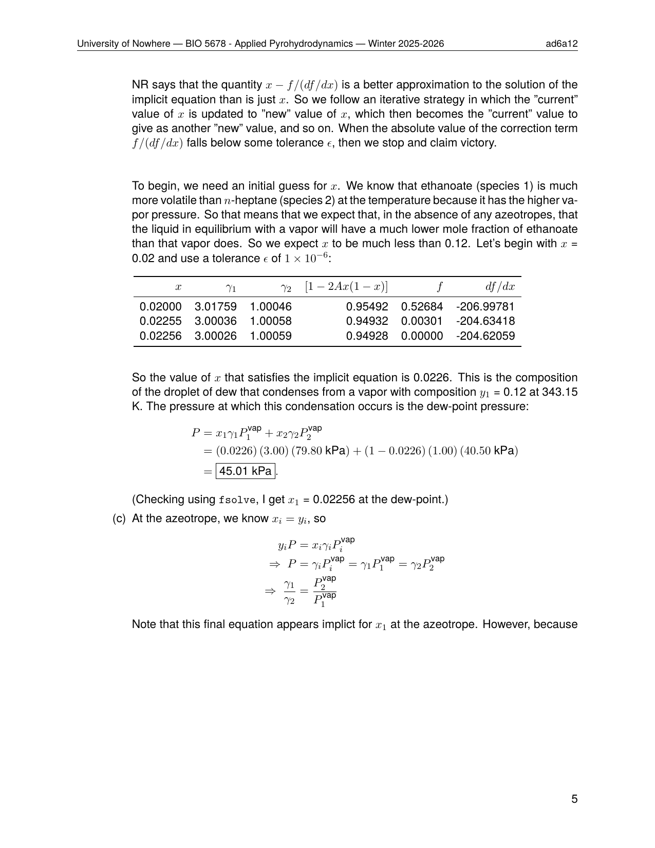
NR says that the quantity $x - f/(df/dx)$ is a better approximation to the solution of the implicit equation than is just $x$.  So we follow an iterative strategy in which the "current" value of $x$ is updated to "new" value of $x$, which then becomes the "current" value to give as another "new" value, and so on.  When the absolute value of the correction term $f/(df/dx)$ falls below some tolerance $\epsilon$, then we stop and claim victory.\\*[1em]

To begin, we need an initial guess for $x$.  We know that ethanoate (species 1) is much more volatile than $n$-heptane (species 2) at the temperature because it has the higher vapor pressure.  So that means that we expect that, in the absence of any azeotropes, that the liquid in equilibrium with a vapor will have a much lower mole fraction of ethanoate than that vapor does.  So we expect $x$ to be much less than \pypp[2]{ydew}. Let's begin with $x$ = \pypp[2]{xinit} and use a tolerance $\epsilon$ of \(\py{tu.format_sig(epsilon, sig=1)}\):

\begin{table}[h]
\begin{center}
\py{nrdf_str}
\end{center}
\end{table}

So the value of $x$ that satisfies the implicit equation is \pypp[4]{xdew}.  This is the composition of the droplet of dew that condenses from a vapor with composition $y_1$ = \pypp[2]{ydew} at \pypp[2]{T}.  The pressure at which this condensation occurs is the dew-point pressure:
\begin{align*}
    P & = x_1\gamma_1P_1^{\rm vap} + x_2 \gamma_2 P_2^{\rm vap}\\
    & = \left(\pypl[4]{xdew}\right)\left(\pypl{gdew[0]}\right)\left(\pypl[2]{Pv[0]}\right) + \left(1-\pypl[4]{xdew}\right)\left(\pypl[2]{gdew[1]}\right)\left(\pypl[2]{Pv[1]}\right)\\
    & = \fbox{\pypp[2]{Pdew}}.
\end{align*}

(Checking using \inl{fsolve}, I get $x_1$ = \pypp[5]{xdew} at the dew-point.)

\item[(c)]  At the azeotrope, we know $x_i = y_i$, so
\begin{align*}
    y_iP & = x_i\gamma_iP_i^{\rm vap}\\
    \Rightarrow\ P& = \gamma_iP_i^{\rm vap} = \gamma_1P_1^{\rm vap} = \gamma_2P_2^{\rm vap}\\
    \Rightarrow\ \frac{\gamma_1}{\gamma_2} &= \frac{P_2^{\rm vap}}{P_1^{\rm vap}}
\end{align*}
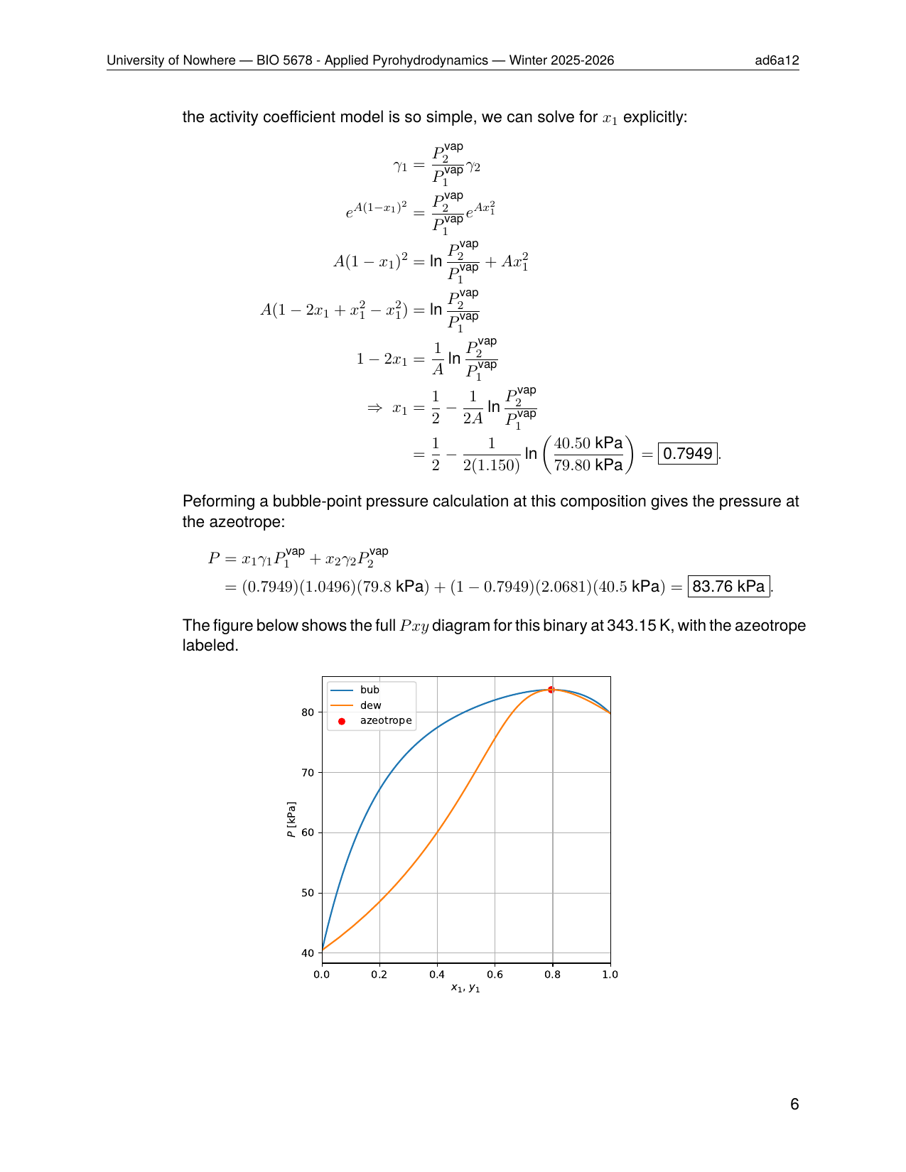
Note that this final equation appears implict for $x_1$ at the azeotrope.  However, because the activity coefficient model is so simple, we can solve for $x_1$ explicitly:
\begin{align*}
    \gamma_1 & = \frac{P_2^{\rm vap}}{P_1^{\rm vap}}\gamma_2\\
    e^{A(1-x_1)^2} & = \frac{P_2^{\rm vap}}{P_1^{\rm vap}}e^{Ax_1^2}\\
    A(1-x_1)^2 & = \ln\frac{P_2^{\rm vap}}{P_1^{\rm vap}} + Ax_1^2\\
    A(1-2x_1+x_1^2-x_1^2) & = \ln\frac{P_2^{\rm vap}}{P_1^{\rm vap}}\\
    1-2x_1 & = \frac{1}{A}\ln\frac{P_2^{\rm vap}}{P_1^{\rm vap}}\\
    \Rightarrow\ x_1 & = \frac{1}{2}-\frac{1}{2A}\ln\frac{P_2^{\rm vap}}{P_1^{\rm vap}}\\
    & = \frac{1}{2}-\frac{1}{2(\pypl[3]{Aij})}\ln\left(\frac{\pypl[2]{Pv[1]}}{\pypl[2]{Pv[0]}}\right) = \fbox{\pypp[4]{xazeo}}.
\end{align*}

Peforming a bubble-point pressure calculation at this composition gives the pressure at the azeotrope:
\begin{align*}
    P & = x_1 \gamma_1 P_1^{\rm vap} + x_2 \gamma_2 P_2^{\rm vap}\\
    & = (\pypl[4]{xazeo})(\pypl[4]{gazeo[0]})(\pypl[1]{Pv[0]}) + (1-\pypl[4]{xazeo})(\pypl[4]{gazeo[1]})(\pypl[1]{Pv[1]}) = \fbox{\pypp[2]{Pazeo}}.
\end{align*}

\IfFileExists{mypxy-<<<serialstr>>>-<<<qno>>>.pdf}{
The figure below shows the full $Pxy$ diagram for this binary at \pypp[2]{T}, with the azeotrope labeled.

\begin{figure}[h]
\begin{center}
\includegraphics[width=0.5\textwidth]{mypxy-<<<serialstr>>>-<<<qno>>>.pdf}
\end{center}
\end{figure}
}{
not showing full $Pxy$ diagram for this binary at \pypp[2]{T} yet
}

\end{enumerate}
\clearpage
\else
\ifgivespace
\clearpage
\noindent (This page left blank for extra space.)
\clearpage
\fi
\fi

This is the most feature-rich problem in the exam. It combines:

• Pint-aware state variables — temperature and vapor pressures are pint.Quantity objects (T = 343.15 * ureg.K, Pv = np.array([79.8, 40.5]) * ureg.kPa), so all P-x-y arithmetic carries units automatically.

• Bubble- and dew-point calculations using the one-constant Margules (OCM) activity-coefficient model, with fsolve from SciPy for the dew-point.

• Newton–Raphson iteration — the NR loop explicitly stores intermediate values in Python lists and then packages them into a pd.DataFrame for inclusion in the solution as a LaTeX table. All quantities going into the dataframe are plain floats; pint magnitudes are extracted with .m consistently in both the loop initialization and the loop body.

• Matplotlib figure — a P-x-y diagram is generated inside the pycode block using the standard fig, ax = plt.subplots(...) pattern and saved with plt.savefig(...); the filename is appended to pythontexFC so pygacity includes it in the build archive. Note that ax.scatter requires a plain scalar for the y-coordinate, so Pazeo.m (not Pazeo) is used when plotting the azeotrope marker.

Problem 4: Ammonia Synthesis Equilibrium (ammonia_synthesis.tex)

\begin{pycode}
REACTOR = Pick.pick_state(
    dict(
        P1={'default':8,'pick':{'between':[7,10],'round':-1}, 'units': ureg.bar}, # bar
        T1={'default':500,'pick':{'between':[480,520], 'round':0}, 'units': ureg.K} # K
    )
)
T = REACTOR.T1
P = REACTOR.P1
d = SandlerProps

nitrogen = Component.from_compound(d.get_compound('nitrogen'), T=298.15 * ureg.K, P=1.0 * ureg.bar)
hydrogen = Component.from_compound(d.get_compound('hydrogen (equilib)'), T=298.15 * ureg.K, P=1.0 * ureg.bar)               
ammonia = Component.from_compound(d.get_compound('ammonia'), T=298.15 * ureg.K, P=1.0 * ureg.bar)                 
components = [nitrogen, hydrogen, ammonia]
n0 = np.array([1.0, 3.0, 0.0])

n0_table = tu.table_as_tex({'Species':[c.as_tex() for c in components], r'$N_{0,i}$ (mol)': n0.tolist()}, sig=3)
rxn = Reaction(components=components)

# need to solve a mock system to get the tex strings
# for equilibrium constants, etc
mock = ChemEqSystem(components=components, N0=n0, T=T, P=P, reactions=[rxn])
ka_calcslines = mock.texgen_kacalculations(sig=5, simplified=True)
logger.debug(f'ka_calcslines: {ka_calcslines}')
mock.solve_implicit(Xinit=[0.5], simplified=True) # single reaction
# report = mock.report()
rxnstr = rxn.as_tex()
sum_nu = rxn.sum_nu()
thermochemicaltable = mock.thermochemicaltable_as_tex(sig=6)
stotable = mock.stoichiometrictable_as_tex(sig=3)
stoprod_activity = rxn.stoichiometric_product_as_tex(base_string=rf'a')
stoprod_pp = rxn.stoichiometric_product_as_tex(base_string=rf'Py', parens=True)
PP = f'P^{{{sum_nu}}}'
stoprod_y = rxn.stoichiometric_product_as_tex(base_string=rf'y')
resultstable = tu.table_as_tex({'Species':[c.as_tex() for c in components],r'$y_i$':mock.ys}, sig=4)

# register answers
AnsSet.register(qno, label=r'\(X_{\rm eq}\)', value=mock.Xeq[0], formatter='{:.5f}')
for y, c in zip(mock.ys, components):
    AnsSet.register(qno, label=rf'\(y_{{\rm {c.as_tex()}}}\)', value=y, formatter='{:.5f}')
\end{pycode}
Consider the following reaction:
\[
\py{rxnstr}
\]

The initial molar feed composition to a reactor is as follows:

\begin{center}
\py{n0_table}
\end{center}

If the reactor is operated at constant \pypp[0]{T} and \pypp[0]{P}, determine the equilibrium mole fractions of each species in the reactor effluent.  You can assume ideal-gas behavior, and that the simplified van't Hoff equation applies for the temperature dependence of the equilibrium constant.

The following thermochemical formation energies at standard state ($P^\circ$ = 1 bar) may be useful:

\begin{center}
\py{thermochemicaltable}
\end{center}

\ifshowsolutions\vspace{1em}\Solutionheader\\

At \pypp[0]{T}, the equilibrium constant for the reaction at the reference temperature $T_0$, followed by the equilibrium constant at the operating temperature $T$, are calculated as follows (via the simplified van't Hoff equation):

\py{ka_calcslines}

We know generally that $K_a$ is the stoichiometric product of activities (i.e., the product of activities each raised to the species' stoichiometric coefficients). So we need to construct the stoichiometric product of the reaction, which is fundamentally expressed using species {\em activities} $a_i$:

\[
a_i = \frac{f_i}{P^\circ}
\]

where $f_i$ is fugacity and $P^\circ$ is the standard state pressure (1 bar).  For an ideal gas, fugacity is equal to partial pressure, so we can write the stoichiometric product as follows:

\[
K_a(T) = \py{stoprod_activity} = \py{stoprod_pp} = \py{PP}\py{stoprod_y}
\]

Note that we have left off the standard state pressure since it is 1 bar; this however requires that we express all pressures in bar when calculating.

To resolve this equation, let's set up the stoichiometric table for the reaction, where we let $X$ be the extent of reaction:

\py{stotable}

Plugging each expression for $y_i$ into the stoichiometric product yields a single equation in the unknown $X$. Solving for $X$ (implicitly) gives:

\[
X = \py{f'{mock.Xeq[0]:.5f}'}
\]

Using this value of $X$, we can compute the equilibrium mole fractions of each species:

\begin{center}
\py{resultstable}    
\end{center}

\clearpage
\fi

This problem demonstrates the deepest integration with the sandler ecosystem. The equilibrium calculation itself is set up on a “mock” system at the picked operating conditions, and the LaTeX for all intermediate steps is generated by monkeypatched methods on ChemEqSystem:

nitrogen = Component.from_compound(d.get_compound('nitrogen'),
                                   T=298.15 * ureg.K, P=1.0 * ureg.bar)
hydrogen = Component.from_compound(d.get_compound('hydrogen (equilib)'),
                                   T=298.15 * ureg.K, P=1.0 * ureg.bar)
ammonia  = Component.from_compound(d.get_compound('ammonia'),
                                   T=298.15 * ureg.K, P=1.0 * ureg.bar)

rxn  = Reaction(components=[nitrogen, hydrogen, ammonia])
mock = ChemEqSystem(components=components, N0=n0, T=T, P=P, reactions=[rxn])

ka_calcslines       = mock.texgen_kacalculations(sig=5, simplified=True)
thermochemicaltable = mock.thermochemicaltable_as_tex(sig=6)
stotable            = mock.stoichiometrictable_as_tex(sig=3)
mock.solve_implicit(Xinit=[0.5], simplified=True)

The operating temperature T and pressure P picked by Pick.pick_state are wrapped in pint units (ureg.K, ureg.bar) before being passed to ChemEqSystem, as are the reference-state conditions for Component.from_compound.

Reaction automatically balances the stoichiometry from the ordered component list (reactants first, products last) using the null-space of the element-count matrix. texgen_kacalculations generates a multi-line align* block showing the simplified van’t Hoff derivation of \(K_a(T)\) from \(K_a(T_0)\) (simplified=True here matches the problem statement, which tells students to use the simplified van’t Hoff equation). solve_implicit is called with the same flag so the numerical answer shown in the solution is consistent with the derivation typeset above it.

Building the Document

From inside the thermo_exam/ directory, run:

pygacity build ThermoExam.yaml

Pygacity generates three student PDFs, three solution PDFs (one per serial), and one answer-set PDF covering all serials.

Output

The build/ directory contains:

• ExamI-{serial}.pdf — student exam for each of the three serials

• ExamI_soln-{serial}.pdf — instructor copy with solutions for each serial

• answerset.pdf — consolidated answer key for all serials

• buildfiles.zip / solnbuildfiles.zip — zipped LaTeX sources

• tex_artifacts.zip — intermediate LaTeX artifacts

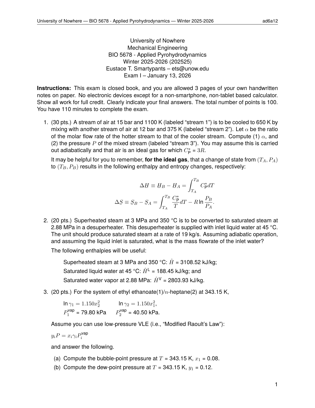
Student exam (serial 00ad6a12) — two pages, problems shown without solutions:

Page 1: problems 1-2 and start of problem 3

Page 2: problem 3 (cont.) and problem 4

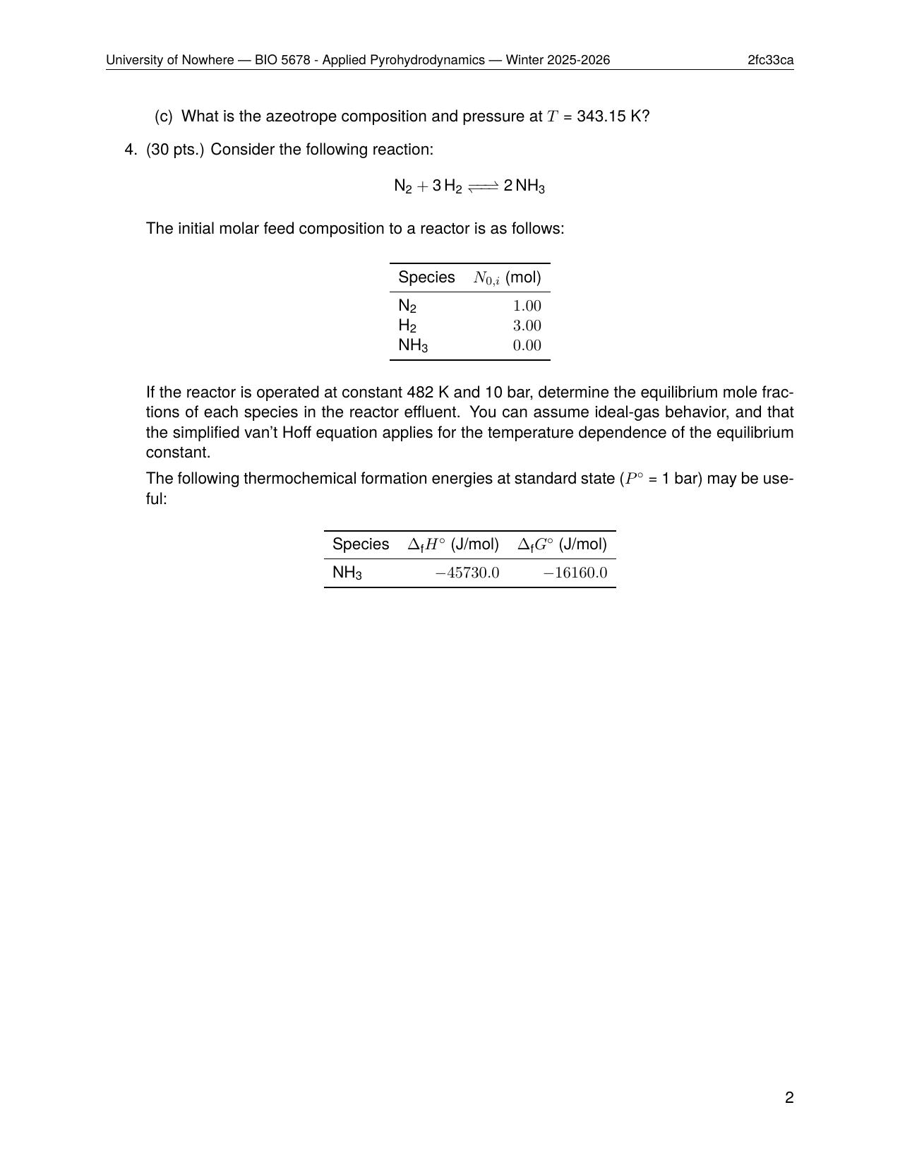
Two serials side by side — the picked values differ between serials (serial-hex: true so they appear as 00ad6a12 and 02fc33ca):

ser. 00ad6a12

ser. 02fc33ca

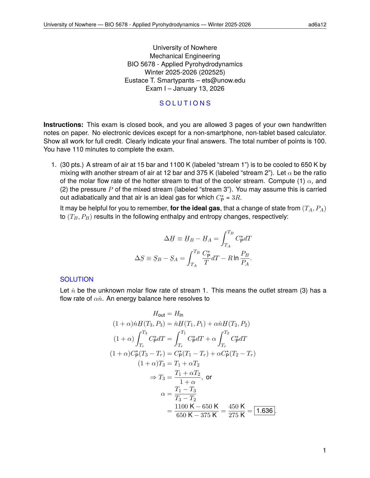
Solutions (serial 00ad6a12, page 1) — full worked solutions with typeset computed values, including the entropy-balance derivation of the mixing pressure:

Solutions (pages 5 and 6) — the VLE problem solution includes the Newton–Raphson iteration table and the P-x-y diagram generated by matplotlib:

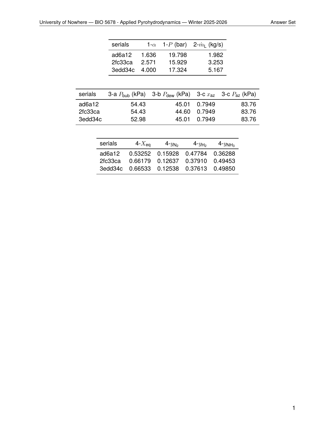
Answer set — one table per question across all three serials. Problem 1 shows \(\alpha\) and \(P_3\); problem 2 shows \(\dot{m}_\mathrm{L}\) (with unit string in the column header). Problem 3 (VLE) shows bubble-point, dew-point, azeotrope composition, and azeotrope pressure. Problem 4 (chemical equilibrium) shows \(X_{\rm eq}\) and the three equilibrium mole fractions: